Introduction

This post describes the notion of an agent minimizing their free-energy and its extension to active inference, which includes the ability for the agent to take action, additionally introducing an expected free-energy. I then derive an approach for applying these methods to reinforcement learning, comparing my approach to another approach in the literature. I then briefly describe predictive coding, a more biologically plausible replacement for backpropagation.

• Minimizing free-energy is exactly what both VAEs and Diffusion models perform. Free-energy is also related to the negative model evidence, and many common objectives minimize this, e.g. cross-entropy and mean-squared loss.

Free-energy

The free-energy principle says that self-organizing systems (e.g. biological systems) can be viewed as minimizing a quantity called the free energy.

There is a mathematically involved derivation of the free-energy principle by assuming that states follow Langevin dynamics along with some other assumptions. For a full description of this approach see Friston (2019).

Assuming the Bayesian brain hypothesis provides another, less involved, route to the concept of the brain minimizing free energy, as will be described in this section. The Bayesian brain hypothesis says: the brain has a generative model describing its beliefs about the world, and this model is updated based on perception.

Specifically, the brain receives sensory data/observation denoted by \(o \in \mathcal{O}\), and it is assumed this data is generated by some underlying process dependent on some cause/latent variable \(x \in \mathcal{X}\). Then the brain’s beliefs are implicitly contained in its generative model \(p(x, o) = p(x) p(o\vert x)\) made up of an explicit:

• prior belief on latent variable \(p(x)\),
• likelihood \(p(o\vert x)\).

After receiving an observation \(o\), the posterior \(p(x\vert o)\) is determined by Bayes rule:

\[p(x\vert o) = \frac{p(x, o)}{p(o)}\]

Typically, however, \(p(o) = \int_{\mathcal{X}} p(x, o) dx\) is intractable, so we consider a variational posterior \(q(x\vert o)\) that we want to effectively approximate \(p(x\vert o)\). The natural objective to achieve this is to minimize the KL-divergence between these distributions, and with some rearranging:

\[\begin{align*} D_{KL}(q(x|o) || p(x|o)) &= D_{KL}(q(x|o) || \frac{p(x, o)}{p(o)})\\ &= D_{KL}(q(x|o) || p(x, o)) + \log(p(o))\\ &\leq D_{KL}(q(x|o) || p(x, o)) =: F(o) \end{align*}\]

where \(F(o)\) is called the variational free energy of observation \(o\), and is a tractable upper bound on this objective. This has shown that updating beliefs in a tractable way can be done by minimizing the variational free energy.

• Variational auto-encoders (VAEs) then follow by letting \(p(o)\) be the data distribution and choosing prior belief \(p(x) := \mathcal{N}(x; 0, I)\) (isotropic Gaussian), and \(p(o|x;\theta)\), \(q(x|o;\phi)\) to be parameterized MVNs, and then applying the reparameterization trick to obtain a low variance estimator of \(\mathbb{E}_{p(o)}[F(o)]\) and applying gradient descent on this estimator.

• Diffusion models follow from a data distribution \(p(o)\) and \(x = (x_1, \ldots, x_T)\), with \(p(x_T)\) an isotropic Gaussian, and generative model \(p(x, o; \theta) = p(x_T) \prod_{t=1}^{T} p(x_{t-1}|x_t; \theta)\) with \(x_0 := o\), and \(q(x|o) = \prod_{t=1}^{T} q(x_t|x_{t-1})\) (i.e. Markov chains in both directions).

  Specifically, there is an exact noising process \(q(x_t|x_{t-1}) := \mathcal{N}(x_t; \sqrt{1 - \beta_t} x_{t-1}, \beta_t I)\) and a parameterized noise-reversing process \(p(x_{t-1}|x_t; \theta) := \mathcal{N}(x_{t-1}; \mu_{\theta}(x_t, t), \Sigma_{\theta}(x_t, t))\). The rest then amounts to minimizing \(\mathbb{E}_{p(o)}[F(o)]\) by using some tricks to find a low variance estimator and applying gradient descent.

The negative model evidence acts as a lower bound on \(F(o)\):

\[\begin{align*} F(o) = D_{KL}(q(x|o)||p(x, o)) &= -\log p(o) + D_{KL}(q(x|o)||p(x|o))\\ &\geq -\log p(o) \end{align*}\]

since the KL-divergence is non-negative. Then, minimizing \(F(o)\) pushes the model evidence \(\log p(o)\) to maximize, i.e. for our perceived observations to match our model.

• Maximizing expected (across a data distribution) model evidence is a common form of objective function in machine learning. For example, cross-entropy does this directly, and the mean squared error is the model evidence under a Gaussian distribution for \(p(o)\).

By manipulating, a more interpretable expression for the free energy can be obtained:

\[F(o) = D_{KL}(q(x|o)||p(x)) - \mathbb{E}_{q(x|o)}[\log p(o|x)]\]

Then minimization of \(F(o)\) incentivizes

• the posterior to be aligned with prior belief, which has a regularizing effect, (left term)
• and the posterior to be accurate at modelling the environment (right term)

Active Inference

Action

Active inference extends the above by including action. The above describes a system updating its beliefs to minimize free energy, but active inference allows the system to also take actions in the environment in order to make its own beliefs come true and hence minimize free energy.

• e.g. an agent may need to remain at a specific temperature, and if their temperature is currently too high, then the agent can either update their model to expect high temperatures (which the brain is stubborn to do, as maintaining the correct temperature is necessary for bodily functions), or they can act in the world in order to change their temperature, such as opening a window.

A systems observational preferences are encoded in its biased prior denoted by \(\tilde{p}(o)\), e.g. \(\tilde{p}(o)\) may assign high probability to high reward observations in the context of RL.

• \(\tilde{p}\) differs from \(p\) in that, for example, \(p(o\vert x)\) is unbiased and models the environment, whereas \(\tilde{p}\) involves the preferences of an agent and depends on its subjective goals.

Future Free Energy

To make effective actions, one must consider the future consequences of actions. To formalize such a notion requires the concept of an expected free energy.

The free energy of the expected future (FEEF) is defined as

\[\mathcal{F} := D_{KL}(q(o, x, \pi) || \tilde{p}(o, x))\]

with \(\tilde{p}(o, x) = \tilde{p}(o) p(x|o)\).

• See Millidge et al. (2020) for a justification of FEEF as a natural extension of the free energy to action.

We decompose \(q(o, x, \pi) = q(\pi) q(o, x \vert \pi)\), with \(q(\pi)\) the prior over policies.

Concretely, one can think of \(o = (o_0, \ldots, o_T)\), \(x = (x_0, \ldots, x_T)\) and \(\pi = (a_0, \ldots, a_{T-1})\) representing the observations, states, and actions respectively for a time horizon of length \(T\).

Rewriting the FEEF using the above decomposition for \(q(o, x, \pi)\) gives:

\[\begin{align*} \mathcal{F} &:= D_{KL}(q(o, x, \pi) || \tilde{p}(o, x))\\ &= \mathbb{E}_{q(o, x, \pi)}[\log(\frac{q(o, x, \pi)}{\tilde{p}(o, x)})]\\ &= \mathbb{E}_{q(o, x, \pi)}[\log(q(\pi)) - (\log(\tilde{p}(o, x)) - \log(q(o, x | \pi)))]\\ &= \mathbb{E}_{q(\pi)}[\log(q(\pi)) - \log(e^{-\mathbb{E}_{q(o, x | \pi)}[\log(q(o, x | \pi)) - \log(\tilde{p}(o, x))]})]\\ &= \mathbb{E}_{q(\pi)}[\log(q(\pi)) - \log(e^{-D_{KL}(q(o, x | \pi) || \tilde{p}(o, x))})]\\ &= D_{KL}(q(\pi) || e^{-D_{KL}(q(o, x | \pi) || \tilde{p}(o, x))})\\ &=: D_{KL}(q(\pi) || e^{-\mathcal{F}_{\pi}}) \end{align*}\]

where \(\mathcal{F}_{\pi} := D_{KL}(q(o, x | \pi) || \tilde{p}(o, x))\), measuring the difference between our preferences (described by \(\tilde{p}(o, x)\)) and the actual trajectories we observe due to a policy \(\pi\).

Hence if we consider minimizing \(\mathcal{F}\) wrt. \(q(\pi)\), then by variational principles, the minimizing solution is \(q(\pi) \propto e^{-\mathcal{F}_{\pi}}\) up to a multiplicative normalizing constant. Hence this says that the best prior policy \(\pi^{*} := \text{argmin}_{\pi} \mathcal{F}_{\pi}\).

We can rewrite \(\mathcal{F}_{\pi}\) in an interpretable form using the approximation \(p(x\vert o) \approx q(x\vert o) \approx q(x\vert o, \pi)\):

\[\begin{align*} \mathcal{F}_{\pi} &:= D_{KL}(q(o, x | \pi) || \tilde{p}(o, x))\\ &= \mathbb{E}_{q(o, x|\pi)}[\log(q(x|\pi)) + \log(q(o|x, \pi)) - \log(\tilde{p}(o)) - \log(p(x|o))]\\ &\approx \mathbb{E}_{q(o, x|\pi)}[\log(q(x|\pi)) + \log(q(o|x, \pi)) - \log(\tilde{p}(o)) - \log(q(x|o, \pi))]\\ &= \mathbb{E}_{q(x|\pi) q(o|x, \pi)}[\log(\frac{q(o|x, \pi)}{\tilde{p}(o)})] - \mathbb{E}_{q(o|\pi) q(x|o, \pi)}[\log(\frac{q(x|o, \pi)}{q(x|\pi)})]\\ &= \mathbb{E}_{q(x|\pi)}[D_{KL}(q(o|x, \pi) || \tilde{p}(o))] - \mathbb{E}_{q(o|\pi)}[D_{KL}(q(x|o, \pi) || q(x|\pi))] \end{align*}\]

and so minimizing \(\mathcal{F}_{\pi}\) means

• The first term, \(\mathbb{E}_{q(x\vert \pi)}[D_{KL}(q(o\vert x, \pi) \| \tilde{p}(o))]\), describing the difference between preferred and expected observations, will be incentivized to decrease.
• The second term, \(\mathbb{E}_{q(o|\pi)}[D_{KL}(q(x|o, \pi) || q(x|\pi))]\), describing the expected information gain under observation, will be incentivized to increase. This can be seen as incentivizing exploration. In the context of reinforcement learning, terms that incentivize exploration must be added ad-hoc, as the idea of value maximization does not explicitly include this, whereas under Active Inference, this idea naturally arises.

Reinforcement Learning

Now consider the special case of reinforcement learning, where for a time horizon of length \(T\),

• States \(x = (s_0, \ldots, s_T)\) of the environment, with \(s_i \in \mathbb{R}^S\).
• Observations \(o = (o_0, \ldots, o_T)\) with \(o_i = (r_i, s_{i+1})\) in the case of RL, since the environment states are given directly to the agent. Reward \(r_i \in \mathbb{R}\).
• Policy \(\pi = (a_0, \ldots, a_T)\), with actions \(a_i \in \mathbb{R}^A\).

forming a Markov Decision Process (MDP). For one step, \((s_i, a_i) \mapsto o_i\) by the environment, with \(o_i = (r_i, s_{i+1})\)

The natural prior which we impose is that \(\tilde{p}(o_i) = \tilde{p}(r_i)\) has a high density for large \(r_i\), such that our agent prefers to achieve high rewards.

By using the properties of an MDP,

\[q(o, x|\pi) = q(x|\pi) q(o|x, \pi) = \prod_{t=0}^{T} q(x_t|x_{t-1}, \pi) q(o_t|x_t, \pi)\]

and also,

\[\tilde{p}(o) = \prod_{t=0}^{T} \tilde{p}(o_t)\]

Recall that we can approximate

\[\mathcal{F}_{\pi} \approx \mathbb{E}_{q(x|\pi)}[D_{KL}(q(o|x, \pi) || \tilde{p}(o))] - \mathbb{E}_{q(o|\pi)}[D_{KL}(q(x|o, \pi) || q(x|\pi))]\]

Using the fact that \(q(o\vert x, \pi) = \prod_{t=0}^{T} q(r_t\vert x_t, a_t)\) (since MDP), \(q(x\vert \pi) = \prod_{t=0}^{T} q(x_t\vert x_{t-1}, a_{t-1})\) and \(\tilde{p}(o) = \prod_{t=0}^{T} \tilde{p}(o_t)\), then the first term can be written

\[\begin{align*} \mathbb{E}_{q(x|\pi)}[D_{KL}(q(o|x, \pi) || \tilde{p}(o))] &= \mathbb{E}_{q(x|\pi)q(o|x, \pi)}[\log(\prod_{t=0}^{T} \frac{q(r_t|x_t, a_t)}{\tilde{p}(r_t)})]\\ &= \sum_{t=0}^{T} \mathbb{E}_{q(x_t|x_{t-1}, a_{t-1}) q(r_t|x_t, a_t)}[\log(\frac{q(r_t|x_t, a_t)}{\tilde{p}(r_t)})]\\ &= \sum_{t=0}^{T} \mathbb{E}_{q(x_t|x_{t-1}, a_{t-1})}[D_{KL}(q(r_t|x_t, a_t) || \tilde{p}(r_t))] \end{align*}\]

and using \(q(x\vert o, \pi) = \frac{q(x\vert \pi)q(o\vert x, \pi)}{q(o\vert \pi)}\) and \(q(o\vert \pi) = \prod_{t=0}^{T} q(x_t(o_t)\vert x_{t-1}(o_{t-1}), a_{t-1}) q(r_t(o_t)\vert x_t(o_t), a_t)\), the second term can be written

\[\begin{align*} \mathbb{E}_{q(o|\pi)}[D_{KL}(q(x|o, \pi) || q(x|\pi))] &= \mathbb{E}_{q(x, o|\pi)}[\log(\frac{q(o|x, \pi)}{q(o|\pi)})]\\ &= \mathbb{E}_{q(x, o|\pi)}[\log(\prod_{t=0}^{T} \frac{q(r_t|x_t, a_t)}{q(x_t|x_{t-1}, a_{t-1}) q(r_t|x_t, a_t)})]\\ &= -\sum_{t=0}^{T} \mathbb{E}_{q(x|\pi) q(o|x, \pi)}[\log(q(x_t|x_{t-1}, a_{t-1}))]\\ &= -\sum_{t=0}^{T} \mathbb{E}_{q(x_{t-1}|x_{t-2}, a_{t-2}) q(x_t|x_{t-1}, a_{t-1})}[\log(q(x_t|x_{t-1}, a_{t-1}))]\\ &= \sum_{t=0}^{T} \mathbb{E}_{q(x_{t-1}|x_{t-2}, a_{t-2})}[H[q(x_t|x_{t-1}, a_{t-1})]] \end{align*}\]

hence we can finally write

\[\mathcal{F}_{\pi} = \sum_{t=0}^{T} \mathcal{F}_{\pi, t}\]

where

\[\mathcal{F}_{\pi, t} := \mathbb{E}_{q(x_t|x_{t-1}, a_{t-1})}[D_{KL}(q(r_t|x_t, a_t) || \tilde{p}(r_t))] - \mathbb{E}_{q(x_{t-1}|x_{t-2}, a_{t-2})}[H[q(x_t|x_{t-1}, a_{t-1})]]\]

In the context of RL, we call \(q(r_t|x_t, a_t)\) the reward model, representing a model of the reward distribution given the state we are in and the actions we take. \(q(x_t|x_{t-1}, a_{t-1})\) is called the transition model and models the next state distribution given the current state and the actions we take.

Implementation

To implement these ideas computationally, we need to pick reward \& transition distributions, alongside a prior \(\tilde{p}(r_t)\). Gaussians are nice in that the KL divergence between two Gaussians has a closed form
expression, and the entropy of a Gaussian is also closed form, which would give a closed form expression for \(\mathcal{F}_{\pi, t}\).

Given this, we choose the reward model \(q(r_t|x_t, a_t) = \mathcal{N}(r_t; f_{\mu}(x_t, a_t), f_{\sigma^2}(x_t, a_t))\) and the transition model \(q(x_t|x_{t-1}, a_{t-1}) = \mathcal{N}(x_t; g_{\mu}(x_{t-1}, a_{t-1}), \text{diag}(g_{\sigma^2}(x_{t-1}, a_{t-1})))\). We represent \(f_{\mu}, f_{\sigma^2}: \mathbb{R}^{S} \times \mathbb{R}^{A} \to \mathbb{R}\) and \(g_{\mu}, g_{\sigma^2}: \mathbb{R}^{S} \times \mathbb{R}^{A} \to \mathbb{R}^{S}\) as neural networks.

A natural prior is \(\tilde{p}(r_t) = \mathcal{N}(r_t; r_{\text{max}}, \alpha^2)\) where \(r_{\text{max}}\) is the maximum reward in the environment and \(\alpha\) is suitably chosen.

Then, we can find

\[D_{KL}(q(o_t|x_t, a_t) || \tilde{p}(o_t)) = \frac{1}{2}\left(\frac{(f_{\mu}(x_t, a_t) - r_{\text{max}})^2 + f_{\sigma^2}(x_t, a_t)}{\alpha^2} + \log\left(\frac{\alpha^2}{f_{\sigma^2}(x_t, a_t)}\right) - 1\right)\]

and

\[H[q(x_t|x_{t-1}, a_{t-1})] = \frac{1}{2} \sum_{i=1}^{S} \log(2\pi e (g_{\sigma^2}(x_{t-1}, a_{t-1}))_i)\]

Hence

\[\begin{align*} \mathcal{F}_{\pi, t} = \frac{1}{2}&\mathbb{E}_{q(x_t|x_{t-1}, \pi)}\left[\frac{(f_{\mu}(x_t, a_t) - r_{\text{max}})^2 + f_{\sigma^2}(x_t, a_t)}{\alpha^2} + \log(\frac{\alpha^2}{f_{\sigma^2}(x_t, a_t)}) - 1\right]\\ &- \frac{1}{2}\mathbb{E}_{q(x_{t-1}|x_{t-2}, \pi)}\left[\sum_{i=1}^{S} \log(2\pi e (g_{\sigma^2}(x_{t-1}, a_{t-1}))_i)\right] \end{align*}\]

• When implementing, the expectances can be approximated by an average over a sufficiently large number of trajectories, sampling stochastically with \(q(x_t\vert x_{t-1}, \pi)\).
• The transition and reward models are pretrained before being used to pick an action.
• At a state, when choosing an action, a group of \(N\) policies (over some horizon \(H\) of timesteps) are randomly sampled (normal dist.) and \(\mathcal{F}_{\pi}\) is evaluated for each, taking the top \(M \ll N\) policies and finding the mean and std across these top policies to then resample new policies and repeat, for a couple iterations, and then finally returning the top policy mean at horizon step \(t=0\), and taking this to be the agent’s next action.
• Details can be found in code: https://github.com/r-gould/active-inference

Tschantz et al. (2020) arrive at a different approximation for \(\mathcal{F}_{\pi}\). I now compare my approach detailed above, and theirs, by implementing my approach into the codebase for their paper, with the same hyperparameters across the two approaches. Saving the rewards across 10 runs for each method and averaging over these runs gives plots:

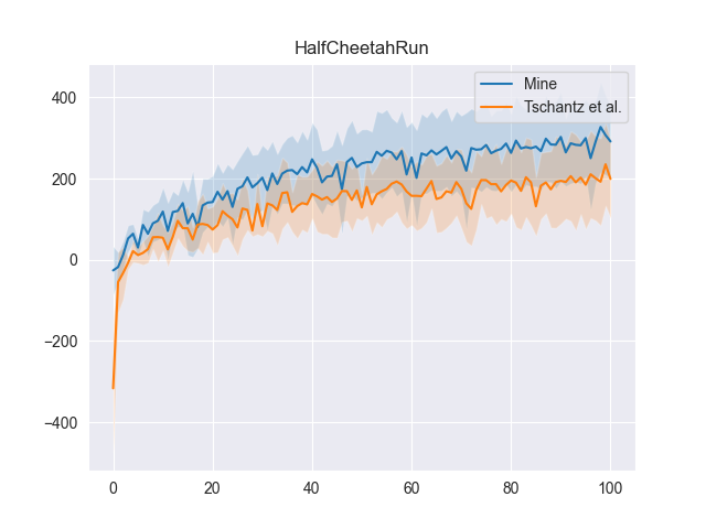
And this approach outperforms with 95% confidence (via. bootstrapping of the \(U\)-statistic wrt. the reward at the final timestep) in both environments.

Code can be found at: https://github.com/r-gould/active-inference

Predictive Coding

Now going back to the case of no action, just perception:

Consider a multi-layer hierarchy described by \(x = (x_1, \ldots, x_L)\) and causal structure

\[x_L \to x_{L-1} \to \cdots \to x_1 \to o\]

which means that \(p(o, x) = \prod_{i=0}^{L} p(x_i\vert x_{i+1})\), with \(x_0 := o\) and \(p(x_L\vert x_{L+1}) := p(x_L)\).

Predictive coding can be derived from here by making normal assumptions. In particular, we let

\[p(x_i|x_{i+1}) := \mathcal{N}(x_i; \mu_i(x_{i+1};\theta_i), \Sigma_i(x_{i+1};\theta_i))\]

and, using the mean field approximation,

\[q(x|o) \approx \prod_{i=1}^{L} q(x_i|o)\]

with \(q(x_i\vert o) := \mathcal{N}(x_i;\hat{\mu}_i, \hat{\Sigma}_i)\).

We can rewrite the free energy as

\[F(o) = D_{KL}(q(x|o)||p(x, o)) = -H[q(x|o)] - \mathbb{E}_{q(x|o)}[\log p(x, o)]\]

The entropy term on the left is nice to evaluate since \(q(x\vert o)\) is the product of Gaussians:

\[\begin{align*} -H[q(x|o)] = -\mathbb{E}_{q(x|o)}[\log q(x|o)] &= -\sum_{i=1}^{L} \mathbb{E}_{q(x_i|o)}[\log q(x_i|o)]\\ &= \sum_{i=1}^{L} H[q(x_i|o)]\\ &= \frac{1}{2} \sum_{i=1}^{L} (n_i + \log(|2\pi \hat{\Sigma}_i|)) \end{align*}\]

with \(x_i \in \mathbb{R}^{n_i}\). See that this is constant with respect to \(\{\theta_i\}_i\) and \(\{\hat{\mu}_i\}_i\).

Assuming that \(\Sigma_i\) is a fixed hyperparameter, the term on the right of \(F(x)\) can be written using a Taylor expansion of \(\log p(x_i\vert x_{i+1})\) about \(x_i = \hat{\mu}_i\), \(x_{i+1} = \hat{\mu}_{i+1}\). Expanding gives

\[\begin{align*} \log p(x_i|x_{i+1}) = \log p(\hat{\mu}_i|\hat{\mu}_{i+1}) &+ (x_i - \hat{\mu}_i)^T \frac{\partial\log p(x_i|x_{i+1})}{\partial x_i}\bigg\rvert_{x_i = \hat{\mu}_i}\\ &+ \frac{1}{2} (x_i - \hat{\mu}_i)^T \frac{\partial^2 \log p(x_i|x_{i+1})}{\partial x_i^2}\bigg\rvert_{x_i = \hat{\mu}_i} (x_i - \hat{\mu}_i) + ... \end{align*}\]

See that \(\mathbb{E}_{q(x_i\vert o)}[x_i-\hat{\mu}_i] = 0\) and \(\frac{\partial^2 \log p(x_i\vert x_{i+1})}{\partial x_i^2} = -\Sigma_i^{-1}\), with third order and higher terms \(0\), and

\[\begin{align*} \mathbb{E}_{q(x_i|o)}[(x_i - \hat{\mu}_i)^T \frac{\partial^2 \log p(x_i|x_{i+1})}{\partial x_i^2}\bigg\rvert_{x_i = \hat{\mu}_i} (x_i - \hat{\mu}_i)] &= -\mathbb{E}_{q(x_i|o)}[\text{tr}((x_i - \hat{\mu}_i)^T \Sigma_i^{-1} (x_i - \hat{\mu}_i))]\\ &= -\mathbb{E}_{q(x_i|o)}[\text{tr}(\Sigma_i^{-1} (x_i - \hat{\mu}_i) (x_i - \hat{\mu}_i)^T)]\\ &= -\mathbb{E}_{q(x_i|o)}[\text{tr}(\Sigma_i^{-1} \hat{\Sigma}_i)] \end{align*}\]

where the last line follows as \(\mathbb{E}\) and \(\text{tr}\) commute, and \(\mathbb{E}_{q(x_i|o)}[(x_i - \hat{\mu}_i) (x_i - \hat{\mu}_i)^T] \equiv \hat{\Sigma}_i\). Therefore the first and second order terms are constant in \(\{\theta_i\}_i\) and \(\{\hat{\mu}_i\}_i\), so the term on the right of \(F(x)\) is

\[-\mathbb{E}_{q(x|o)}[\log p(x, o)] = -\sum_{i=0}^{L} \mathbb{E}_{q(x|o)}[\log p(x_i|x_{i+1})] = -\sum_{i=0}^{L} \log p(\hat{\mu}_i|\hat{\mu}_{i+1}) + \text{const}\]

with \(\hat{\mu}_0 := x_0\). Hence the free energy is

\[\begin{align*} F(o) &= -\sum_{i=0}^{L} \log p(\hat{\mu}_i|\hat{\mu}_{i+1}) + \text{const}\\ &= \frac{1}{2} \sum_{i=0}^{L} ((\hat{\mu}_i - \mu_i(\hat{\mu}_{i+1};\theta_i))^T \Sigma_i(\hat{\mu}_{i+1};\theta_i)^{-1} (\hat{\mu}_i - \mu_i(\hat{\mu}_{i+1};\theta_i)) + \log(|2\pi \Sigma_i(\hat{\mu}_{i+1};\theta_i)|)) + \text{const}\\ &=: \frac{1}{2} \sum_{i=0}^{L} (\epsilon_i^T \Sigma_i^{-1} \epsilon_i + \log(|2\pi \Sigma_i|)) + \text{const} \end{align*}\]

with \(\epsilon_i := \hat{\mu}_i - \mu_i(\hat{\mu}_{i+1};\theta_i)\).

• In the case of \(\Sigma_i = I\), then minimizing the free energy amounts to minimizing \(\sum_{i=0}^{L} \lVert \epsilon_i \rVert^2\), pushing \(\hat{\mu}_i\) and \(\mu_i(\hat{\mu}_{i+1};\theta_i)\) towards eachother. \(\hat{\mu}_{i+1}\) from the layer \(i+1\) is used to predict \(\hat{\mu}_i\) for layer \(i\).

Free energy can then be minimized by optimizing over \(\{\theta_i\}_i\) and \(\{\hat{\mu}_i\}_i\).

• Optimizing over \(\{\theta_i\}_i\), which parameterize \(p(o, x)\), can be thought of as learning the relationship between hidden states and observations,
• and optimizing over \(\{\hat{\mu}_i\}_i\), which parameterize \(q(x\vert o)\), can be thought of as improving perception, getting better at inferring the underlying hidden state given an observation.

We can use gradient descent to perform this optimization, with gradients

\[\frac{\partial F}{\partial \theta_i} = -\left(\frac{\partial \mu_i}{\partial \theta_i}\right)^T \Sigma_i^{-1} \epsilon_i\] \[\frac{\partial F}{\partial \hat{\mu}_i} = \Sigma_i^{-1} \epsilon_i - 1\{i \geq 1\} \frac{\partial \mu_{i-1}}{\partial \hat{\mu}_i} \Sigma_{i-1}^{-1} \epsilon_{i-1}\]

with \(1\{\; \cdot \;\}\) the indicator function.

• The update of \(\theta_i\) depends just on the error \(\epsilon_i\) involving \(\hat{\mu}_i\), and \(\hat{\mu}_{i+1}\) from the layer above.
• The update of \(\hat{\mu}_i\) requires \(\epsilon_i\) too but also the gradient information \(\frac{\partial \mu_{i-1}}{\partial \hat{\mu}_i}\) and the error \(\epsilon_{i-1}\) involving \(\hat{\mu}_i\), and \(\hat{\mu}_{i-1}\) from below.

i.e. these updates are local.

• Millidge et al. (2020) shows that with a reversed causal structure (for the backward pass) of

  \[o \to x_1 \to \cdots \to x_L\]

  and \(\Sigma_i = I\), then at the equilibrium point with \(\frac{\partial F}{\partial \hat{\mu}_i} = 0\) and loss \(\mathcal{L} := \frac{1}{2} (T - \mu_L)^2\) for targets \(T\), the fixed points of the errors are \(\epsilon_i^* = \frac{\partial \mathcal{L}}{\partial \mu_i}\) if one chooses \(\hat{\mu}_L := T\). Additionally we have \(\frac{\partial F}{\partial \theta_i} = -\frac{\partial \mathcal{L}}{\partial \theta_i}\).

• The notable observation here is that through local updates, one can converge at exactly what backpropagation does (which requires global gradient information). Due to this locality, predictive coding is considered a biologically-plausible learning algorithm for the brain. TODO: Describe this part better, go into more details about correspondence between predictive coding and backprop